Chapter 10 Applying POSEIDON
10.1 Flexible Scenario
In this section we go through a proper attempt at using POSEIDON straight from translating data and knowledge about the fishery to calibration and validation. It is still all fake data, of course, but I hope it is useful as an exercise.
In this section we will focus on the Flexible scenario. It is very similar to the Abstract scenario we have dealt with in the previous chapters but it has a few modifications to make it easy to add multiple populations, regulations and ports.
The downside of it is that these modifications are still unsupported by the GUI, so most of the edits will have to be done on the YAML file themselves.
You can run the Flexible scenario just by selecting it in the scenario screen.
When started it looks and feels much like the Abstract example except for having two ports on by default.
It pays to take a look at the YAML file of the scenario since we are supposed to work primarily on this:
Flexible:
  allowFriendshipsAcrossPorts: false
  biologyInitializer:
    Diffusing Logistic:
      carryingCapacity: '5000.0'
      differentialPercentageToMove: '0.001'
      grower:
        Independent Logistic Grower:
          steepness: uniform 0.6 0.8
      maxInitialCapacity: '1.0'
      minInitialCapacity: '0.0'
      percentageLimitOnDailyMovement: '0.01'
      speciesName: Species 0
  cheaters: false
  fisherDefinitions:
  - departingStrategy:
      Fixed Rest:
        hoursBetweenEachDeparture: '12.0'
    destinationStrategy:
      Imitator-Explorator:
        alwaysCopyBest: true
        automaticallyIgnoreAreasWhereFishNeverGrows: false
        automaticallyIgnoreMPAs: false
        backtracksOnBadExploration: true
        dropInUtilityNeededForUnfriend: '-1.0'
        ignoreEdgeDirection: true
        ignoreFailedTrips: false
        maxInitialDistance: -1.0
        objectiveFunction:
          Hourly Profit Objective:
            opportunityCosts: true
        probability:
          Adaptive Probability:
            explorationProbability: '0.2'
            explorationProbabilityMinimum: '0.01'
            imitationProbability: '1.0'
            incrementMultiplier: '0.02'
        stepSize: uniform 1.0 10.0
    discardingStrategy: No Discarding
    fishingStrategy:
      Until Full With Day Limit:
        daysAtSea: '5.0'
    fuelTankSize: '100000.0'
    gear:
      Random Catchability:
        gasPerHourFished: '5.0'
        meanCatchabilityFirstSpecies: '0.01'
        meanCatchabilityOtherSpecies: '0.01'
        standardDeviationCatchabilityFirstSpecies: '0.0'
        standardDeviationCatchabilityOtherSpecies: '0.0'
    gearStrategy: Never Change Gear
    holdSize: '100.0'
    hourlyVariableCost: '0.0'
    initialFishersPerPort:
      Port 0: 50
      Port 1: 50
    literPerKilometer: '10.0'
    logbook: No Logbook
    regulation: Anarchy
    speedInKmh: '5.0'
    tags: ''
    usePredictors: false
    weatherStrategy: Ignore Weather
  gasPricePerLiter: '0.01'
  habitatInitializer: All Sand
  mapInitializer:
    Simple Map:
      cellSizeInKilometers: '10.0'
      coastalRoughness: '4.0'
      depthSmoothing: '1000000.0'
      height: '50.0'
      maxLandWidth: '10.0'
      width: '50.0'
  mapMakerDedicatedRandomSeed: null
  market:
    Fixed Price Market:
      marketPrice: '10.0'
  networkBuilder:
    Equal Out Degree:
      allowMutualFriendships: true
      degree: '2.0'
      equalOutDegree: true
  plugins: [
    ]
  portInitializer:
    Random Ports:
      numberOfPorts: '2.0'
  portSwitching: false
  weatherInitializer:
    Constant Weather:
      temperature: '30.0'
      windOrientation: '0.0'
      windSpeed: '0.0'
The main difference from the Abstract scenario is the presence of fisherDefinitions which is just a list (in yaml you can tell it’s a list because each item starts with -) of populations.
A population is described by the usual behavioural rules (strategies) as well as their number by port listed in initialFishersPerPort.
10.2 How to use data in POSEIDON
As with all models, there are 3 basic uses for data in POSEIDON. It can be used either as:
- Input: basically by using what we know to set some parameters directly (number of boats, geography, port locations and the like)
- Calibration: we use the data to select some parameters indirectly. For example we know how much was landed for the past 5 years and we want to find the catchability parameter that generate the same time series.
- Validation: we don’t use the data to set any parameters, we only use it after everything else is set to make sure the model makes sense (basically “out-of-sample” prediction error from statistics)
Sometimes the way to use a particular datum is clear, other times it is up to the modeller to figure it out.
It should be said that often we just don’t have enough data. There are three basic approaches on how to setup the model when data doesn’t exist:
- Guess: use expert knowledge or some basic theoretical result to model certain parameters. This is of course a much weaker parametrization than using real data but it is sometimes necessary
- Sensitivity Analysis: run the model multiple times for a large enough confidence interval around the parameters you do not know much about. This tends to be hard to do when there are a lot of uknowns unless you use a smart search strategy
- Worst Case Scenario: like sensitivity analysis but looking specifically for the worst possible combination of parameters. This is useful when we need to provide policy suggestions. It’s at least a way to know whether we can be sure not to make things worse off by intervening.
POSEIDON of course has a lot of variables (say, boat speed or fuel consumption) and one might wonder why using it in data poor scenarios where a bio-economic model would only require at most a guess on global fishing mortality.
Three reasons.
First, it is often the case that we do have some knowledge about some details of the fishery which we wouldn’t be able to use when aggregating everything back to global fishing mortality (perhaps the overall number of boats, the price premium for plate-size fish or which port catches most of what).
Second, we might care deeply about the distribution of benefits and costs both in terms of human populations as well as geographical effects on the biology which call for a model that at least tracks these details.
Third, a global fishing mortality guess papers over all the actual things we need to make a guess about. POSEIDON, when presented with absolute lack of any knowledge, forces you to be explicit about everything you do not know.
At its simplest POSEIDON need to have some knowledge about the following:
- Market
- The ex-vessel price of fish caught
- Geography:
- A decent enough bathymetry to distribute the fish in
- Management:
- The policies in place (and if calibrating then also the changes in policies over time)
- Fishing Fleet:
- # of vessels, vessel capacity and speed
- Gear type/catchability (usually by calibration)
- Operational costs (fuel, logistics)
- Maximum possible effort (max number of days out, max length of a trip)
- Biology:
- For each species at least
- Some form of carrying capacity
- Current biomass
- Some depth ranges where these fish live
- For each species at least
10.3 The Peter Snapper Fishery
Let’s assume we want to study a basic made-up fishery: the Indonesian Petern Snapper fishery. I would classify this as a medium-data fishery, since we have a decent knowledge of its human side while knowing basically nothing biologically (after all, 80% of the catch comes from unassessed fisheries according to Costello et al. 2012). Let’s start with some very basic knowledge:
- The fishery is located around Bali, say between lat-long \((114.5,-6.9)\) and (127.6, -12.85)
- It’s a single species fishery
- We know too little about age structure so this will be a biomass-only model
We can already add some of this knowledge in.
First, we want to add the right map. We have seen how to download maps in section 5; fortunately this particular map comes with POSEIDON in directory: inputs/indonesia/indonesia_latlong.csv. Let’s modify the mapInitializer:
  mapInitializer:
    From File Map:
      gridWidthInCell: '70.0'
      header: true
      latLong: true
      mapFile: /home/carrknight/code/POSEIDON/inputs/indonesia/indonesia_latlong.csv
The number of cells is set to 70 since that generates cells approximately 30km wide. This is useful as it allows us to ignore things like congestion or boats moving between cells as they fish.
We can also use a more detailed biology parameter; we still don’t know its parameters but we can prepare for them:
  biologyInitializer:
    Single Species Biomass Normalized:
      biomassSuppliedPerCell: false
      carryingCapacity: '500000000'
      differentialPercentageToMove: '0.001'
      grower:
        Common Logistic Grower:
          steepness: '0.5'
      initialBiomassAllocator:
        Random Allocator:
          maximum: '1'
          minimum: '0'
      initialCapacityAllocator:
        Equal Allocation:
          constantValue: '1.0'
      percentageLimitOnDailyMovement: '0.01'
      speciesName: Peter Snapper
      unfishable: false
This biology initializer looks complicated but it just involves a few things:
carryingCapacitycontrols the \(K\) of the overall fishery.Common Logistic Growermeans that recruitment is global (a single logistic growth for all the cells).steepnessis the malthusian growth of the fishinitialBiomassAllocatordefines the current biomass ratio \(\frac{\text{Biomass Now}}{K}\)initialCapacityAllocatordefines which areas of the ocean are habitable by this speciesdifferentialPercentageToMoveandpercentageLimitOnDailyMovementdefine the speed of fish movement. These numbers imply a very slow moving fish
So far we don’t know enough to fill any of them.
Finally, since we don’t have the resources to field a serious behavioural survey, let’s stick with agents acting as simple explore-exploit-imitate agents with a flat 20% chance of exploration. It proved quite effective in our West Coast application.
    destinationStrategy:
      Imitator-Explorator:
        alwaysCopyBest: true
        automaticallyIgnoreAreasWhereFishNeverGrows: true
        automaticallyIgnoreMPAs: false
        backtracksOnBadExploration: true
        dropInUtilityNeededForUnfriend: '-1.0'
        ignoreEdgeDirection: true
        ignoreFailedTrips: false
        maxInitialDistance: -1.0
        objectiveFunction:
          Hourly Profit Objective:
            opportunityCosts: true
        probability:
          Fixed Probability:
            explorationProbability: '0.2'
            imitationProbability: '1.0'
        stepSize: uniform 1.0 10.0
Notice that we set automaticallyIgnoreAreasWhereFishNeverGrows to true. This has no effect now, but what it does is that it prevents fishers from wasting time exploring areas where the depth or habitat makes it impossible for Peter Snapper to live.
Once all those modifications are done, the model looks like this:
This is yaml file now:
Flexible:
  allowFriendshipsAcrossPorts: false
  biologyInitializer:
    Single Species Biomass Normalized:
      biomassSuppliedPerCell: false
      carryingCapacity: '500000000'
      differentialPercentageToMove: '0.001'
      grower:
        Common Logistic Grower:
          steepness: '0.5'
      initialBiomassAllocator:
        Random Allocator:
          maximum: '1'
          minimum: '0'
      initialCapacityAllocator:
        Equal Allocation:
          constantValue: '1.0'
      percentageLimitOnDailyMovement: '0.01'
      speciesName: Peter Snapper
      unfishable: false
  cheaters: false
  fisherDefinitions:
  - departingStrategy:
      Fixed Rest:
        hoursBetweenEachDeparture: '12.0'
    destinationStrategy:
      Imitator-Explorator:
        alwaysCopyBest: true
        automaticallyIgnoreAreasWhereFishNeverGrows: true
        automaticallyIgnoreMPAs: false
        backtracksOnBadExploration: true
        dropInUtilityNeededForUnfriend: '-1.0'
        ignoreEdgeDirection: true
        ignoreFailedTrips: false
        maxInitialDistance: -1.0
        objectiveFunction:
          Hourly Profit Objective:
            opportunityCosts: true
        probability:
          Fixed Probability:
            explorationProbability: '0.2'
            imitationProbability: '1.0'
        stepSize: uniform 1.0 10.0
    discardingStrategy: No Discarding
    fishingStrategy:
      Until Full With Day Limit:
        daysAtSea: '5.0'
    fuelTankSize: '100000.0'
    gear:
      Random Catchability:
        gasPerHourFished: '5.0'
        meanCatchabilityFirstSpecies: '0.01'
        meanCatchabilityOtherSpecies: '0.01'
        standardDeviationCatchabilityFirstSpecies: '0.0'
        standardDeviationCatchabilityOtherSpecies: '0.0'
    gearStrategy: Never Change Gear
    holdSize: '100.0'
    hourlyVariableCost: '0.0'
    initialFishersPerPort:
      Port 0: 50
      Port 1: 50
    literPerKilometer: '10.0'
    logbook: No Logbook
    regulation: Anarchy
    speedInKmh: '5.0'
    tags: ''
    usePredictors: false
    weatherStrategy: Ignore Weather
  gasPricePerLiter: '0.01'
  habitatInitializer: All Sand
  mapInitializer:
    From File Map:
      gridWidthInCell: '70.0'
      header: true
      latLong: true
      mapFile: /home/carrknight/code/oxfish/inputs/indonesia/indonesia_latlong.csv
  mapMakerDedicatedRandomSeed: null
  market:
    Fixed Price Market:
      marketPrice: '10.0'
  networkBuilder:
    Equal Out Degree:
      allowMutualFriendships: true
      degree: '2.0'
      equalOutDegree: true
  plugins: [
    ]
  portInitializer:
    Random Ports:
      numberOfPorts: '2.0'
  portSwitching: false
  weatherInitializer:
    Constant Weather:
      temperature: '30.0'
      windOrientation: '0.0'
      windSpeed: '0.0'
10.4 Adding boats to the right ports
The fleet is the major component of POSEIDON and the one that require the most knowledge. There are a several ways to learn about it:
- Surveys: interviewing fishers (or, more likely, interviewing people who interview fishers)
- Logbook data: if reliable, logbook data contains basically all the possible human data observable
- VMS / Satellite: an alternative when logbook data is unreliable or not available
- Formulas: there are quite a lot of handrules about how much a boat is expected to catch given its size or consume in gas according to their engine power, these could be used in the model.
There are some basic facts about snapper fisheries in Indonesia we can use immediately:
- Snapper sells on average for about 40,000 IDR per kg
- Diesel costs about 10,000 IDR per liter
Let’s also assume the Peter Snapper fishery is a licensed fishery and that:
- 25 boats fish from Benoa
- 50 boats fish from Kupang
Let’s add this to the model. First, let’s just agree to use IDR as currency. We want to add prices and gas costs:
Let’s define the ports now, in lat-long coordinates. You can grab them from google maps (an advantage in using lat-long coordinates). POSEIDON tries to place the port correctly if the coordinates are slightly too far inland or at sea, so there is no reason to worry about too much precision. POSEIDON however will throw an error if two ports share the same cell. In that case, merge the ports or increase the map resolution.
portInitializer:
List of Ports:
ports:
Benoa: 115.238843,-8.799605
Kupang: 123.586249,-10.148044
usingGridCoordinates: falseNotice usingGridCoordinates is set to false. When that is set to true you are to provide the coordinates in terms of POSEIDON grid instead of lat-long.
Finally, let’s place fishers in the right port:
We can run the model now; it’s still very incomplete but at least there are the right number of boats and ports.
This the YAML file so far:
Flexible:
biologyInitializer:
Single Species Biomass Normalized:
biomassSuppliedPerCell: false
carryingCapacity: '500000000'
differentialPercentageToMove: '0.001'
grower:
Common Logistic Grower:
steepness: '0.5'
initialBiomassAllocator:
Random Allocator:
maximum: '1'
minimum: '0'
initialCapacityAllocator:
Equal Allocation:
constantValue: '1.0'
percentageLimitOnDailyMovement: '0.01'
speciesName: Peter Snapper
unfishable: false
cheaters: false
fisherDefinitions:
- departingStrategy:
Fixed Rest:
hoursBetweenEachDeparture: '12.0'
destinationStrategy:
Imitator-Explorator:
alwaysCopyBest: true
automaticallyIgnoreAreasWhereFishNeverGrows: true
automaticallyIgnoreMPAs: false
backtracksOnBadExploration: true
dropInUtilityNeededForUnfriend: '-1.0'
ignoreEdgeDirection: true
ignoreFailedTrips: false
maxInitialDistance: -1.0
objectiveFunction:
Hourly Profit Objective:
opportunityCosts: true
probability:
Fixed Probability:
explorationProbability: '0.2'
imitationProbability: '1.0'
stepSize: uniform 1.0 10.0
discardingStrategy: No Discarding
fishingStrategy:
Until Full With Day Limit:
daysAtSea: '5.0'
fuelTankSize: '100000.0'
gear:
Random Catchability:
gasPerHourFished: '5.0'
meanCatchabilityFirstSpecies: '0.01'
meanCatchabilityOtherSpecies: '0.01'
standardDeviationCatchabilityFirstSpecies: '0.0'
standardDeviationCatchabilityOtherSpecies: '0.0'
gearStrategy: Never Change Gear
holdSize: '100.0'
hourlyVariableCost: '0.0'
initialFishersPerPort:
Benoa : 25
Kupang: 50
literPerKilometer: '10.0'
logbook: No Logbook
regulation: Anarchy
speedInKmh: '5.0'
tags: ''
usePredictors: false
weatherStrategy: Ignore Weather
gasPricePerLiter: '10000'
habitatInitializer: All Sand
mapInitializer:
From File Map:
gridWidthInCell: '70.0'
header: true
latLong: true
mapFile: /home/carrknight/code/oxfish/inputs/indonesia/indonesia_latlong.csv
mapMakerDedicatedRandomSeed: null
  market:
    Fixed Price Market:
      marketPrice: '40000.0'
networkBuilder:
Equal Out Degree:
allowMutualFriendships: true
degree: '2.0'
equalOutDegree: true
plugins: [
]
  portInitializer:
    List of Ports:
      ports:
        Benoa: 115.238843,-8.799605
        Kupang: 123.586249,-10.148044
      usingGridCoordinates: false
portSwitching: false
weatherInitializer:
Constant Weather:
temperature: '30.0'
windOrientation: '0.0'
windSpeed: '0.0'10.5 Adding knowledge about boat operations
Imagine that we get hold of an expert and get some basic answers on how boats in the fishery work. In particular:
- Boats can hold at most 15t of fish before being too full to continue
- Trips never last more than 10 days (when families back to port start getting angry or the boat runs out of cigarettes)
- Boats cruise at about 8.5 knots (about 16kph)
- Fishing is done by droplining
Let’s also assume we manage to back out (by formula, by asking the expert or by sheer guess) some logistics about the fishery:
- Boats consume about 3\(\frac {l}{\text{km}}\) of diesel when cruising
- Each hour spent fishing consumes 70l of diesel (keeping boat steady and so on)
We can add all these informations in. Start with the boat information in the fisherDefinitions
We can run the model again. We have pretty realistic boats now but unfortunately we still have no idea about what the biology looks like.
10.6 The simplest possible biology input
Trevor A. Branch lists 15 “fisheries controversies” on his website. Number 2 is Can we use catch data alone to make inferences about fishery stock status?. This is in contrast to the standard way of assessing stocks which requiers the time series of both landings and effort, as in chapter 11 of Haddon (2011).
The classic technique for those brave enough, like us for the Peter Snapper fishery, to do stock assessment with landings alone is by using the catch-MSY method (Martell and Froese 2013).
The basic idea is that if you have some landings and some prior on what the stock looks like now, there are only a few combinations of \(K\) (carrying capacity) and \(r\) (malthusian growth) that qualify.
Let’s try our best with what we have (がんばれ).
Imagine having decent landing data (in kg) for the past 10 years.
## # A tibble: 10 x 1
## Landings
## <dbl>
## 1 30765238.
## 2 23983452.
## 3 19843028.
## 4 16148729.
## 5 13046744.
## 6 10867591.
## 7 9221522.
## 8 7628867.
## 9 7041957.
## 10 6200139.Looks like a nasty drop from a 30,000t fishery to a 6,200t fishery in the span of 10 years.
We can go lookup on FishBase the properties of the Peter Snapper (except of course that it’s an imaginary fish). Let’s just pretend it claims the Peter Snapper to be of Low resilience (like, say, the flame snapper). This is useful because it means we can probably bound the malthusian growth parameter \(r \in (.2,.5)\)
While we are on FishBase we can also take a look at the depth range of the fish. Let’s say it gives us a range between 30 and 800 meters.
To use catch-MSY we need some bounds on the current and initial (10 years ago) depletion rate. Let’s say 10 years ago we guess the biomass was at 70-80% of \(K\) as the fishery was still young. Given the big drop in landings we assume the biomass remaining somewhere between 5-25% of \(K\).
These are all the inputs we need for catch-MSY. There are many R libraries implementing the method but I like the original code that came with the paper the most.
It looks something like this:
and when run it gives us a guessed \(K\) and \(r\):
geom. mean r = 0.372
geom. mean k = 110749315 Which we can put in the model. We add \(k\) as carrying capacity, \(r\) as steepness and depth ranges in the initial capacity allocation (which defines which areas are livable, more precisely: it defines how carrying capacity is to be distributed geographically).
The initialBiomassAllocator object contains our current biomass ratio guess: \(\frac{B_t}{K}\). We argued before that number is \(\frac{B_t}{K} \in (.2,.05)\) now and $ (.8,.7)$ ten years ago.
We will start with the 10 year old guess which will be helpful for calibration later.
biologyInitializer:
Single Species Biomass Normalized:
biomassSuppliedPerCell: false
carryingCapacity: '110749315'
differentialPercentageToMove: '0.001'
grower:
Common Logistic Grower:
steepness: '0.372'
initialBiomassAllocator:
Random Allocator:
maximum: '.8'
minimum: '.7'
initialCapacityAllocator:
Depth Allocator:
delegate:
Equal Allocation:
constantValue: '1.0'
maxDepth: '800.0'
minDepth: '30.0'
percentageLimitOnDailyMovement: '0.01'
speciesName: Peter Snapper
unfishable: falseHere’s how the input file looks like now:
Flexible:
biologyInitializer:
Single Species Biomass Normalized:
biomassSuppliedPerCell: false
carryingCapacity: '110749315'
differentialPercentageToMove: '0.001'
grower:
Common Logistic Grower:
steepness: '0.372'
initialBiomassAllocator:
Random Allocator:
maximum: '.8'
minimum: '.7'
initialCapacityAllocator:
Depth Allocator:
delegate:
Equal Allocation:
constantValue: '1.0'
maxDepth: '800.0'
minDepth: '30.0'
percentageLimitOnDailyMovement: '0.01'
speciesName: Peter Snapper
unfishable: false
cheaters: false
fisherDefinitions:
- departingStrategy:
Fixed Rest:
hoursBetweenEachDeparture: '12.0'
destinationStrategy:
Imitator-Explorator:
alwaysCopyBest: true
automaticallyIgnoreAreasWhereFishNeverGrows: true
automaticallyIgnoreMPAs: false
backtracksOnBadExploration: true
dropInUtilityNeededForUnfriend: '-1.0'
ignoreEdgeDirection: true
ignoreFailedTrips: false
maxInitialDistance: -1.0
objectiveFunction:
Hourly Profit Objective:
opportunityCosts: true
probability:
Fixed Probability:
explorationProbability: '0.2'
imitationProbability: '1.0'
stepSize: uniform 1.0 10.0
discardingStrategy: No Discarding
fishingStrategy:
Until Full With Day Limit:
daysAtSea: '10.0'
fuelTankSize: '100000.0'
gear:
Random Catchability:
gasPerHourFished: '70.0'
meanCatchabilityFirstSpecies: '0.01'
meanCatchabilityOtherSpecies: '0.01'
standardDeviationCatchabilityFirstSpecies: '0.0'
standardDeviationCatchabilityOtherSpecies: '0.0'
gearStrategy: Never Change Gear
holdSize: '15000.0'
hourlyVariableCost: '0.0'
    initialFishersPerPort:
      Benoa : 25
      Kupang: 50
literPerKilometer: '3.0'
logbook: No Logbook
regulation: Anarchy
speedInKmh: '16.0'
tags: ''
usePredictors: false
weatherStrategy: Ignore Weather
gasPricePerLiter: '10000'
habitatInitializer: All Sand
mapInitializer:
From File Map:
gridWidthInCell: '70.0'
header: true
latLong: true
mapFile: /home/carrknight/code/oxfish/inputs/indonesia/indonesia_latlong.csv
mapMakerDedicatedRandomSeed: null
market:
Fixed Price Market:
marketPrice: '40000.0'
networkBuilder:
Equal Out Degree:
allowMutualFriendships: true
degree: '2.0'
equalOutDegree: true
plugins: [
]
portInitializer:
List of Ports:
ports:
Benoa: 115.238843,-8.799605
Kupang: 123.586249,-10.148044
usingGridCoordinates: false
portSwitching: false
weatherInitializer:
Constant Weather:
temperature: '30.0'
windOrientation: '0.0'
windSpeed: '0.0'10.7 Calibrating Catchability
One key parameter for any fishery model is catchability: the percentage of fish available in an area caught by one hour of effort. You can’t get this from surveys and you can’t use stock assessment estimates (since they are usually not geographical or at least not at the level we care about).
Catchability needs to be calibrated.
Calibration simply mean that we want to tune some parameters (catchability) to minimize the distance between model output and reality. In our case, the only data we have is 10 years of landings. We want to modify catchability (\(q\)) until the landings in the model are as close as possible to the data. This is a minimization problem: \[ q^* = \arg \min_q \sum^{10}_{t=1} \text{Landings}_t-\text{ModelLandings}_t \]
Now, there are a million different minimization routines one can use and feel free to use any of them. Currently in POSEIDON I am experimenting with EVA which is in java and distributed together with POSEIDON. You can use it by calling (in linux/mac):
while in Windows:
gradlew.bat optimizerI will however immediately confess that most optimization so far in POSEIDON have happened through by coding them in Java rather than using the gui so the options here are quite limited.
- We need to choose an optimization method. For simple non-linear problems I select NelderMeadSimplex and set its population size to 5 (which makes it faster but only good at local searches).
- Eva is a multi-purpose optimization platform. We need to feed it a POSEIDON problem. Select in
ProblemtheSimpleProblemWrapperand from there selectSimple Problem. From there you can select (by looking for the “open file” icon) and look in the POSEIDON folder for/eva/flexible.yaml
- We need to:
- point the scenario towards a
csvfile containing the landings observed, inLanding Data - set catchability bounds (keeping the default \(\in (0.00001,0.005)\))
- point to the scenario file we want to calibrate, in
Scenario File - set up how many different kind of agents we need to calibrate (just 1 in our case), in
Populations - define the name of the species, in
Species Name - point to where to store all our runs and associated errors for debugging purposes, in
Summary File
- point the scenario towards a
- Set up a few details before running the calibration
- Collect best and solution at each time step in the
Statisticstab - In the
Problem,SimpleProblemWrapperset up how many simulations to run in parallel if your computer can handle them
- Collect best and solution at each time step in the
- Finally run the calibration and wait
Each calibration runs somewhat differently but I’d expect a result such as this:
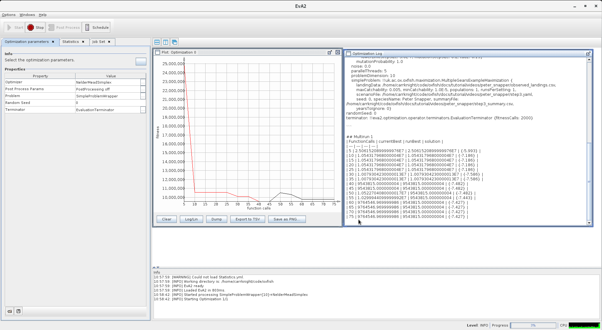
The fitness represents the distance between the two time series (about 10,000t off over 10 years). The solution in the log is the catchability value we are looking for. Eva scales it between -10 and 10. The catchability \(q\) given Eva suggestion \(x\) then is:
\[ q = \frac{(x+10)}{20} \times (0.005-0.00001) \]
Since the solution quoted by Eva is −7.427 the catchability guessed is: \(0.000641964\)
Finally we can add this number in the scenario:
gear:
Random Catchability:
gasPerHourFished: '70.0'
meanCatchabilityFirstSpecies: '0.000641964'
meanCatchabilityOtherSpecies: '0.01'
standardDeviationCatchabilityFirstSpecies: '0.0'
standardDeviationCatchabilityOtherSpecies: '0.0'Giving us the final scenario:
Flexible:
biologyInitializer:
Single Species Biomass Normalized:
biomassSuppliedPerCell: false
carryingCapacity: '110749315'
differentialPercentageToMove: '0.001'
grower:
Common Logistic Grower:
steepness: '0.372'
initialBiomassAllocator:
Random Allocator:
maximum: '.8'
minimum: '.7'
initialCapacityAllocator:
Depth Allocator:
delegate:
Equal Allocation:
constantValue: '1.0'
maxDepth: '800.0'
minDepth: '30.0'
percentageLimitOnDailyMovement: '0.01'
speciesName: Peter Snapper
unfishable: false
cheaters: false
fisherDefinitions:
- departingStrategy:
Fixed Rest:
hoursBetweenEachDeparture: '12.0'
destinationStrategy:
Imitator-Explorator:
alwaysCopyBest: true
automaticallyIgnoreAreasWhereFishNeverGrows: true
automaticallyIgnoreMPAs: false
backtracksOnBadExploration: true
dropInUtilityNeededForUnfriend: '-1.0'
ignoreEdgeDirection: true
ignoreFailedTrips: false
maxInitialDistance: -1.0
objectiveFunction:
Hourly Profit Objective:
opportunityCosts: true
probability:
Fixed Probability:
explorationProbability: '0.2'
imitationProbability: '1.0'
stepSize: uniform 1.0 10.0
discardingStrategy: No Discarding
    fishingStrategy:
      Until Full With Day Limit:
        daysAtSea: '10.0'
fuelTankSize: '100000.0'
    gear:
      Random Catchability:
        gasPerHourFished: '70.0'
meanCatchabilityFirstSpecies: '0.000641964'
meanCatchabilityOtherSpecies: '0.01'
standardDeviationCatchabilityFirstSpecies: '0.0'
standardDeviationCatchabilityOtherSpecies: '0.0'
gearStrategy: Never Change Gear
holdSize: '15000.0'
hourlyVariableCost: '0.0'
initialFishersPerPort:
Benoa : 25
Kupang: 50
literPerKilometer: '3.0'
logbook: No Logbook
regulation: Anarchy
speedInKmh: '16.0'
tags: ''
usePredictors: false
weatherStrategy: Ignore Weather
gasPricePerLiter: '10000'
habitatInitializer: All Sand
mapInitializer:
From File Map:
gridWidthInCell: '70.0'
header: true
latLong: true
mapFile: /home/carrknight/code/oxfish/inputs/indonesia/indonesia_latlong.csv
mapMakerDedicatedRandomSeed: null
market:
Fixed Price Market:
marketPrice: '40000.0'
networkBuilder:
Equal Out Degree:
allowMutualFriendships: true
degree: '2.0'
equalOutDegree: true
plugins: [
]
portInitializer:
List of Ports:
ports:
Benoa: 115.238843,-8.799605
Kupang: 123.586249,-10.148044
usingGridCoordinates: false
portSwitching: false
weatherInitializer:
Constant Weather:
temperature: '30.0'
windOrientation: '0.0'
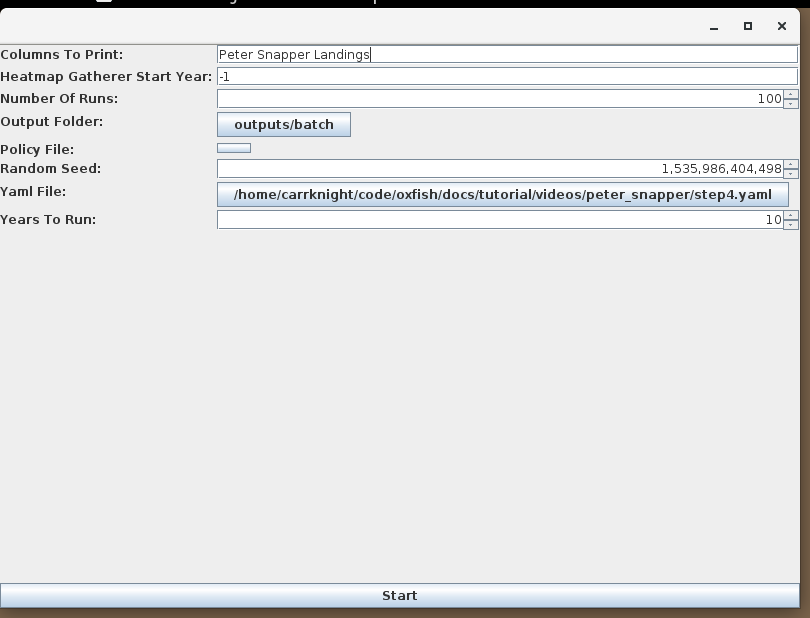
windSpeed: '0.0'We can look at our calibration now by running it in batch 100 times and plotting its landings. We saw how to run batches in chapter 7. This is just a straightforward application of it.
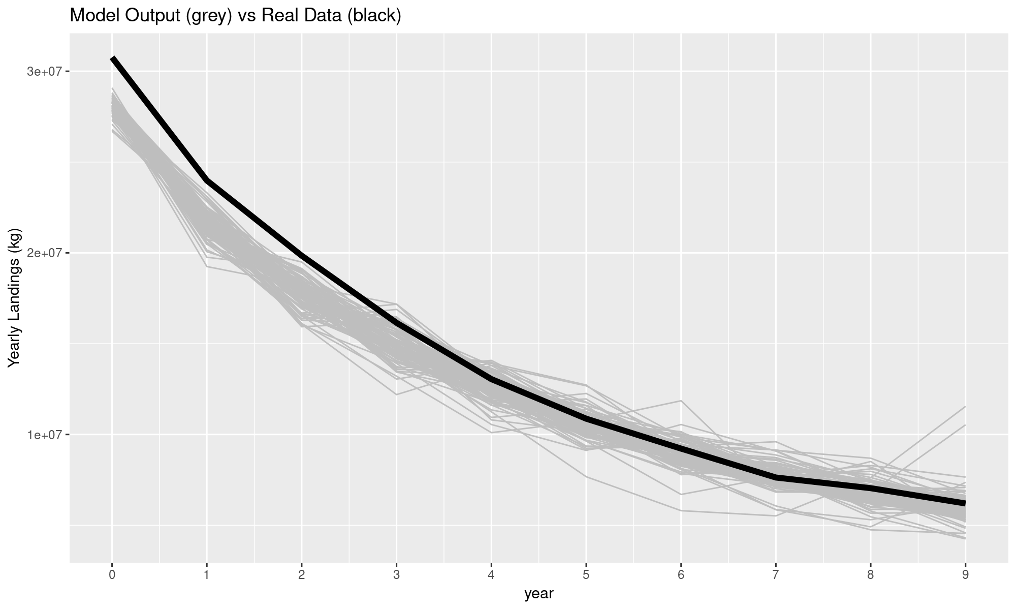
And here’s how the model output (grey lines) compares to the “real world” (bold black line). It’s quite close in the later years but not so much very early on.
I can now reveal that the “real” 10 years of landings were actually also coming from POSEIDON and we can check how far off the real values were from the “real” scenario:
  biologyInitializer:
    Single Species Biomass Normalized:
      biomassSuppliedPerCell: false
      carryingCapacity: '1.25E8'
      differentialPercentageToMove: '0.001'
      grower:
        Common Logistic Grower:
          steepness: '0.33'
      initialBiomassAllocator:
        Random Allocator:
          maximum: '.8'
          minimum: '.7'
      initialCapacityAllocator:
        Depth Allocator:
          delegate:
            Equal Allocation:
              constantValue: '1.0'
          maxDepth: '800.0'
          minDepth: '30.0'
      percentageLimitOnDailyMovement: '0.01'
      speciesName: Peter Snapper
      unfishable: false
gear:
Random Catchability:
gasPerHourFished: '72.0'
meanCatchabilityFirstSpecies: '6.2E-4'
meanCatchabilityOtherSpecies: '0.01'
standardDeviationCatchabilityFirstSpecies: '0.0'
standardDeviationCatchabilityOtherSpecies: '0.0'
gearStrategy: Never Change Gear
holdSize: '15000.0'
hourlyVariableCost: '0.0'
initialFishersPerPort:
Benoa : 25
Kupang: 50
literPerKilometer: '3.5'As you can see \(K\) and \(r\) were not perfectly estimated (in particular for \(K\) we are about 10,000t too low which explains the gap between real and calibrated output). We also had errors in gas consumption, mileage and catchability although all these were minor. Overall, quite a nice match given how little data we used.
10.8 Validation
Validation refers to the model matching data for which it was not calibrated against. This gives us an intuitively more honest prediction error estimation. It is particularly useful for two reasons:
- We are afraid of over-fitting to the data we have
- We have multiple valid assumptions and want to choose the one that predicts best
In this example we used up all the data for calibration so we can’t do validation without gathering more. An alternative would have been finding \(K\), \(r\) and \(q\) on a subset of the data (say, the first 8 years) and check the quality of the model by its prediction of year 9 and 10.
10.9 References
References
Costello, Christopher, Daniel Ovando, Ray Hilborn, Steven D. Gaines, Olivier Deschenes, and Sarah E. Lester. 2012. “Status and solutions for the world’s unassessed fisheries.” Science 338 (6106): 517–20. https://doi.org/10.1126/science.1223389.
Haddon, Malcolm. 2011. Modelling and Quantitative Methods in Fisheries. 2nd ed. Boca Raton, FL: Crc Press-Taylor & Francis Group.
Martell, Steven, and Rainer Froese. 2013. “A simple method for estimating MSY from catch and resilience.” Fish and Fisheries 14 (4): 504–14. https://doi.org/10.1111/j.1467-2979.2012.00485.x.